Knn Regression
In Machine Learning sometimes data is missing and has to be accounted for. There are multiple ways to take care of this data, such as averaging over all the values, simply removing the data corresponding to that feature vector, or even by just filling it with a randomly chosen value.
However, this provides a problem when you’re dealing with smaller data sets, as it can skew your data, and even cause over fitting, if you don’t have enough data with similar feature vectors. Therefore, another way to take care of it is to use regression techniques to get a “best guess” of the value based on the other feature vectors. One way to do this is with the use of K-Nearest Neighbors Regression.
K-Nearest Neighbors
K-Nearest Neighbors is a classification algorithm that works in many dimensional spaces. It works on the principle of classifying data based on the distance between feature vectors, and groups them all together. For continuous features, there are multiple ways to calculate these distances, as follows:
- Euclidean Distance:
- Manhattan Distance:
- Minkowski Distance:
However, for discrete data, you should use the Hamming Distance
- Hamming Distance:
Where in the above instances, is the number of features in each feature vector. The KNN algorithm is easy to implement, with pseudocode in Python below
# c: Data to classify
# dataSet: Labeled data
# k: Number of nearest neighbors
def KNN(c, dataSet, k):
    neighbors = []
    for data in dataSet:
        d = Distance(data, c)
        if len(neighbors) < k:
            neighbors.append([d, data])
        else if d < max(item[0] for item in neighbors):
            max_d = max(item[0] for item in neighbors)
            indx = next(vec for vec in neighbors if max_d in vec)
            neighbors[indx] = [d, data]
    return neighbors
which returns the k nearest neighbors back to where the function was called
so a decision can be made on what to do with the neighbors and labelling the
unlabeled data c.
The Distance function is determined on how you want to implement it based on the above types of distances. The overall speed of this algorithm is , where is the number of features per vector and is the number of unlabeled data.
It is a good idea to choose an odd value for k rather than even. For example,
let’s say that a value of k = 4 was chosen, and you’re labelling a user’s
favorite music genre based on their other favorite songs. The KNN algorithm could
possibly return 2 nearest neighbors for “pop music” and 2 for “rock and roll.”
This leads to a problem on attemping to label the data, since it is an even split.
However, with choosing an odd value such as k = 3 or k = 5, you can label the
user based on a “majority rules” type of instance, where if the algorithm returned
2 for “rock and roll” and 1 for “pop,” you would label them as “rock and roll.”
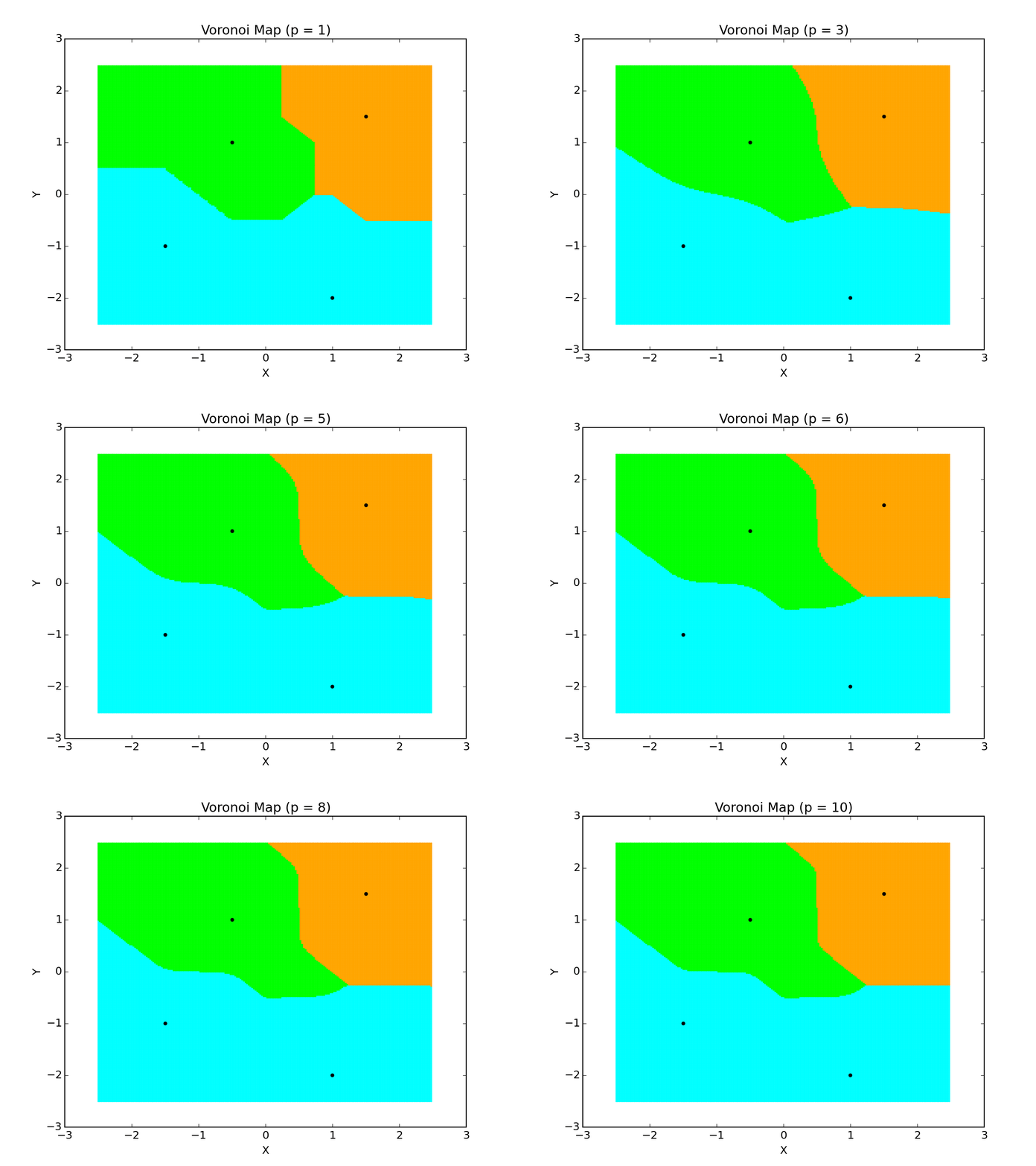
An example of how influences the regions of classification can be seen in the example below, which is a Voronoi Diagram of different values for that I wrote in Python for 4 points. The colors denote the labeling/regions.

There isn’t much change since the points are spaced decently far apart for the region, but you can see some changes in the labeling based on the value of .
KNN Regression
Now that we have the KNN algorithm, we can see how to use this in the instance of regression to interpolate for missing values.
Essentially what would happen, is if we have some unknown/missing feature in the feature vector , we would simply calculate the K nearest neighbors of without using feature , and get some subset of feature vectors which have been found to be closely related to that value.
From here, there are two options:
- Make the average of the values of in the neighbors
- Take the weighted distance of in the neighbors to decide the value in
Either will work. Most commonly the first is used, and provides a good enough representation of the data such that you can now use the whole data set with less worry about over fitting or throwing away useful data.
