Titanic Deaths
This dataset came from kaggle which stated to use random forests for prediction.
Random Forests
Random forests are not much different from decision trees, with the difference being that they are an agglomeration of decision trees, or in other words a “forest.”
In using this method, it allows for it to reduce the variance of the estimate by avaeraging together many estimates. For example, to train trees, we take subsets of the data, chosen randomly with replacement, and then compute the ensemble
where is the tree. This technique is known as “bagging” or “bootstrap aggregating.”
In implementing this algorithm, too high of a value of will be prone to over-fitting while too small a value will be prone to underfitting.
Titanic Deaths
My code can be found here.
The features that were provided in the data are listed as follows:
| Label | Description |
|---|---|
| survival | Survival (0 = No; 1 = Yes) |
| pclass | Passenger Class (1 = 1st; 2 = 2nd; 3 = 3rd) |
| name | Name |
| sex | Sex |
| age | Age |
| sibsp | Number of Siblings/Spouses Aboard |
| parch | Number of Parents/Children Aboard |
| ticket | Ticket Number |
| fare | Passenger Fare |
| cabin | Cabin |
| embarked | Port of Embarkation (C = Cherbourg; Q = Queenstown; S = Southampton) |
As with most datasets, this one had missing features as well. The important ones were age and fare. To fix this, the average age from the training set as well as the agerage fare. These averages were then applied to the missing values in both the training set and the test set. The average was not taken from the test set as to not introduce any future knowledge into the set.
After cleaning up the data, it was ready to analyze. As in the movie for the Titanic, they’re asking to have the women and children be put into the rescue boats first. Therefore, my initial hypothesis before exploring the data is that sex and age will be the dominant factors for who survives or not.
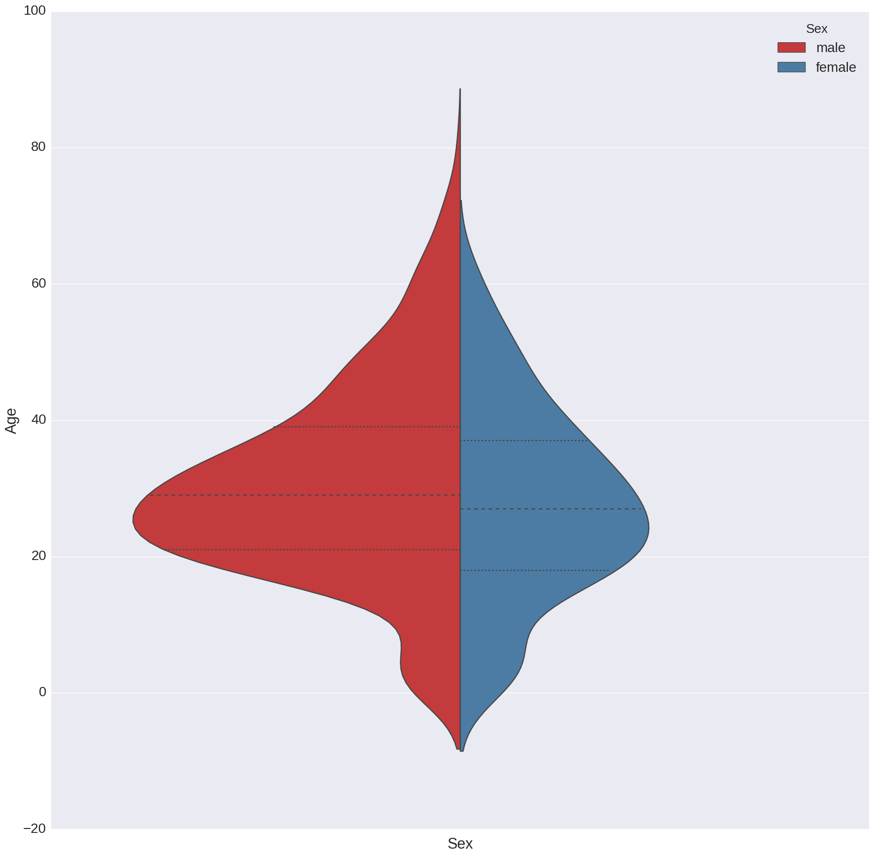
The above figure shows a violin plot of a distribution of ages for males and feamels abord the Titanic. The thicker line shows the median, and the thinner lines show the quartiles for the ages. The height of each has been scaled by the observed number of counts in the test set. As this shows, there are more men than women on the boat, and also had a more diverse age range.
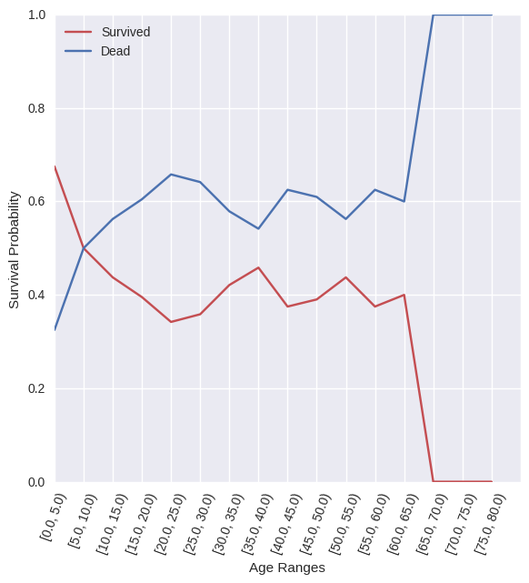
This figure shows the probability of surviving over different age ranges for those on the boat. This seems to show what the above hypothesis proposed, where the age is a dominant factor in determining survival.
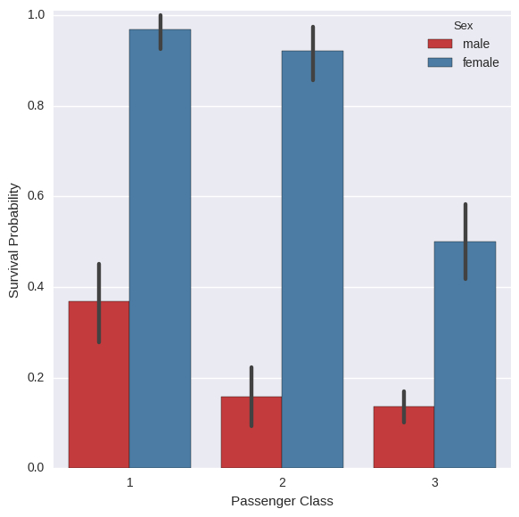
Instead of just looking at gender, I decided to look at both gender and class status. As is blatantly clear from this above figure, the probability of a woman surviving was much greater than men.
However, in this figure, we can see another important distinction, and that’s class. The higher class, the larger chance of survival. Because of this, the fares were looked at as well, and the effect they had on survival. The idea was that the higher class people would pay more in fares.
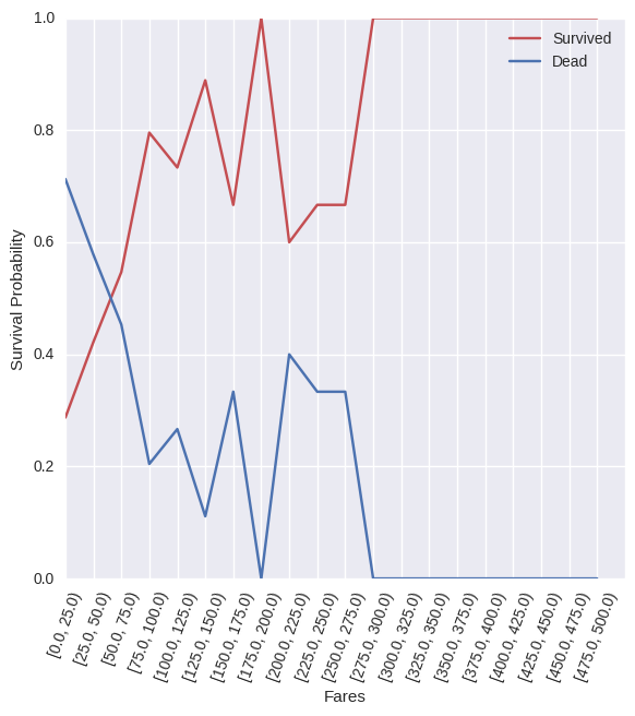
As this figure shows, there is a large distinction between the fares. At the lower fare prices, the chance of dying was above that of surviving. However, as the fares went up, past around $45, the chance of survival was much greater than dying.
As this figure has a large separation between the values, it was suspected that the fares would also have a dominant role in determining who is going to survive or not on the Titanic.
The feature vectors that were used in this simulation were
- Passenger Class (
pclass) - Sex (
sex) - Age (
age) - Number of Siblings/Spouses Aboard (
sibsp) - Number of Parents/Children (
parch) - Passenger Fare (
fare)
The other features such as cabin where they were staying would also be useful, but this would have required external data which was not availble. This could be helpful as the people further away from the life boats would not have had as easy of a time as reaching them, and those that were closer would.
Results
Before going over the results, the description for this stated “Know that a score of 0.79 - 0.81 is doing well on this challenge, and 0.81-0.82 is really going beyond the basic models!” This will be the baseline of the implementation provided.
The results of my implementation averaged on 0.84 for the accuracy. The table with the accuracy measurements can be seen below.
| Prediction | precision | recall | f1-score | support |
|---|---|---|---|---|
| 0 | 0.86 | 0.89 | 0.88 | 267 |
| 1 | 0.79 | 0.74 | 0.77 | 151 |
| avg/total | 0.84 | 0.84 | 0.84 | 418 |
From the above quote, 84% accuracy is a good fit for the data. Again, as stated above, the cabins would have been able to increase this accuracy, however there were too many that did not have this information, thus making most interpolation techniques almost useless, and not able to provide decent results.
From this fit, we can also see which features were most dominant in the random forest. The “ranking” value is essentially how much “weight” is given to that feature in the tree’s decision process.
| Feature | Ranking |
|---|---|
| Fare | 0.297525 |
| Sex | 0.267874 |
| Age | 0.259869 |
| Class | 0.090779 |
| SibSp | 0.049662 |
| ParCh | 0.034291 |
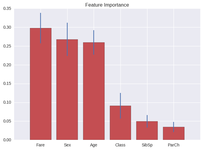
As the above shows, sex and age were large contributing factors in the decision making. However, as was suspected from the fares plot, the fare was also a large factor. This is most probably due to the fact that the 1st class could afford the more expensive fares, and they were the most likely ones to be saved.