Credit Card Fraud
Logistic Regression
Logistic Regression is a classification algorithm for classifying discrete classes. In other words, we want to classify data such that we get or for the class. This can be transformed into a Multi-class Classifier, such that , but for now we will just take the approach of it being a single classifier.
Logistic Regression has a hypothesis function that produces values in the range . This is due to the fact that the equation for the hypothesis is
Which is also known as the “Sigmoid Function.” The Sigmoid Function has the shape
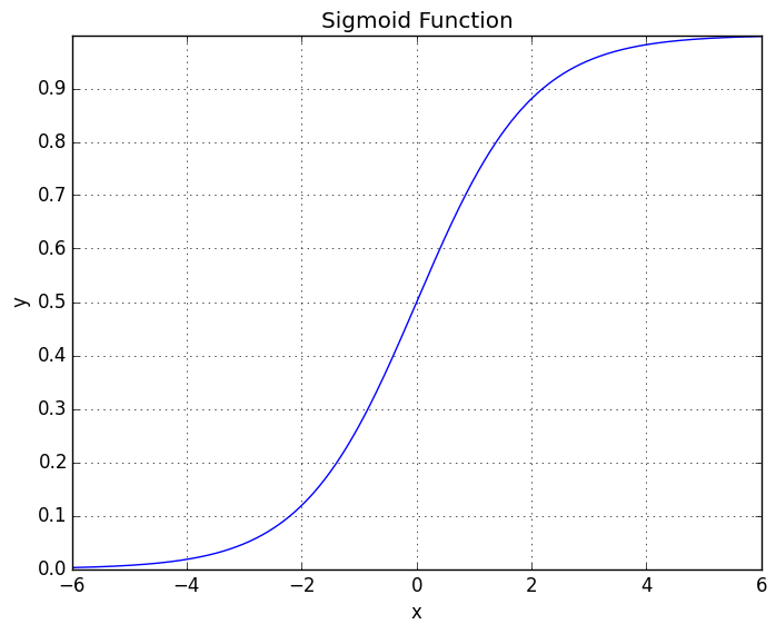
which asymptotes at and . Just like with Linear Regression, we need to fit the parameters to the data to produce the results. We can interpret the output of as being the “probability” that on a given .
In order to classify the data, we need a decision boundary, which is the point at which we will decide if we classify the data as or . What we can do, is we can predict that if and if .
From the picture of the Sigmoid Function, we can see that for values in the positive domain, and in the negative domain.
Therefore, we can say that whenever . And conversly, we can say that it will be less than whenever .
Cost Function
We can define our cost function for Logistic Regression as being
Which makes sense as a cost function to use. Because if and , then the cost is . However, as , we get . This is good because we want our classifier to pay a large cost if it gets it wrong.
We can simplify this cost function into a single equation, instead of a piecewise equation, as being
Which we are able to do since . So it cancels out the appropriate opposing factor. This gives our cost function as being
And, again, to get the values of we want to solve
For which we will use Gradient Descent. In simplifying the like before, we get
which is the same as we had before. Therefore, we can use the same function as we did for Gradient Descent to get the minimization of .
Regularized Logistic Regression
Regularizing helps with overfitting. In order to implement regularization, we need to change the cost function. For example, we now have
With the second term being the Regularization Term, and is the regularization parameter, which controls the parameters of fitting the training set well, and secondly keeping the parameters small.
If is very large , then we will start penalizing all of the parameters and we will have all of the parameters tend towards zero. And if is very small , then it will have very little effect on regularizing the data and is back to prone to overfitting again. Therefore, we need a “good choice” in choosing .
We also need to rederive since it has now changed. However, not much has changed so we can simply write it as
Which ignores the first “offset” term since there is no need to regularize it, and it stays the same as before. However, we can write all ’s as a single equation by rearranging the two to give
This update can be used for Linear Regression as well.
Support Vector Machines
Sometimes called a “Large Margin Classifier.” This means that it attempts to maximize the margin spacing between the two classes, by maximizing the distance between the closest and , while still separating the two classes.
It does this with the cost function
where we want for and for .
Linear SVM is implemented in Scikit-Learn by using sklearn.svm.LinearSVC,
with the documentation can be found here here.
Naive Bayes classification
Naive Bayes use Bayes’ Theorem with the “naive” assumption of independence between every pair of features. Given a class variable and a dependent feature vector through , Bayes’ theorem states the following relationship:
Using the naive independence assumption that
for all ’s. This relationship can be simplified into
Since is constant for any of the inputs, we can simplify it further by stating
Which we can then write down the classifier as
Upsampling
Up Sampling is a technique that is used for when one class of the data is drastically unevenly represented in the data. To help with this, upsampling continually resamples from the underrepresented class until both data sets are represented relatively equal. This is done for the training set.
It is important that this is only done for the training set since you want the test data to remain relatively the same unevenness as the original data when predicting.
For example, in the case of credit card fraud, it only happens in a fraction of a percent of credit card transactions. Therefore, for the best “total accuracy” if we just let it train on the normal data, it would essentially ignore the fradulent cases since they’re not as represented. We changed this by giving it a roughly 50/50 distribution between the two classes, resampling from the data.
However, when running our trained model on the test set, we want to see how it will perform on the “real world data,” so the test set was not upsampled at all.
Credit Card Fraud Detection
All three of these techniques can be used for classifying credit card fraud. The dataset was download from here. It’s important to note that the data was anonymized so that there was no identifiable information in it. Therefore, it was impossible to tell what the “dominant property” was in identifying a transaction as credit card fraud.
The code that was used for this classification problem can be found here.
In order to perform the classification on this data, the following steps were taken:
- Separate the data into two classes
- Take 20% of the data from both classes as the “test set”
- Build the training set with Upsampling
- Independently shuffle both data sets
But first, we have to look at and explore the data
%matplotlib inline
from __future__ import print_function, division
import datetime
import os
import sys
import matplotlib.pyplot as plt
import numpy as np
import seaborn as sns
sns.set(color_codes=True)
import pandas as pd
from sklearn.svm import LinearSVC
from sklearn.linear_model import LogisticRegressionCV
from sklearn.naive_bayes import GaussianNB
from sklearn.metrics import classification_report
from scipy import stats, integrate
# Gets the path/library with my Machine Learning Programs and adds it to the
# current PATH so it can be imported
LIB_PATH = os.path.dirname(os.getcwd()) # Goes one parent directory up
LIB_PATH = LIB_PATH + "/Library/" # Appends the Library folder to the path
sys.path.append(LIB_PATH)
from ML_Alg import LogisticRegression, UpSample
from f_io import ReadCSV
And we can read in the data
data_file = "creditcard.csv"
DIR = os.getcwd() + "/data/"
FILE = DIR + data_file

x, y = ReadCSV(FILE)
card_data = pd.read_csv(FILE)
Check for missing data in the dataset
card_data.isnull().sum()
Time      0
V1        0
V2        0
V3        0
V4        0
V5        0
V6        0
V7        0
V8        0
V9        0
V10       0
V11       0
V12       0
V13       0
V14       0
V15       0
V16       0
V17       0
V18       0
V19       0
V20       0
V21       0
V22       0
V23       0
V24       0
V25       0
V26       0
V27       0
V28       0
Amount    0
Class     0
dtype: int64
Learn what the columns mean
card_data.describe()
| Time | V1 | V2 | V3 | V4 | V5 | V6 | V7 | V8 | V9 | ... | V21 | V22 | V23 | V24 | V25 | V26 | V27 | V28 | Amount | Class | |
|---|---|---|---|---|---|---|---|---|---|---|---|---|---|---|---|---|---|---|---|---|---|
| count | 284807.000000 | 2.848070e+05 | 2.848070e+05 | 2.848070e+05 | 2.848070e+05 | 2.848070e+05 | 2.848070e+05 | 2.848070e+05 | 2.848070e+05 | 2.848070e+05 | ... | 2.848070e+05 | 2.848070e+05 | 2.848070e+05 | 2.848070e+05 | 2.848070e+05 | 2.848070e+05 | 2.848070e+05 | 2.848070e+05 | 284807.000000 | 284807.000000 |
| mean | 94813.859575 | 3.919560e-15 | 5.688174e-16 | -8.769071e-15 | 2.782312e-15 | -1.552563e-15 | 2.010663e-15 | -1.694249e-15 | -1.927028e-16 | -3.137024e-15 | ... | 1.537294e-16 | 7.959909e-16 | 5.367590e-16 | 4.458112e-15 | 1.453003e-15 | 1.699104e-15 | -3.660161e-16 | -1.206049e-16 | 88.349619 | 0.001727 |
| std | 47488.145955 | 1.958696e+00 | 1.651309e+00 | 1.516255e+00 | 1.415869e+00 | 1.380247e+00 | 1.332271e+00 | 1.237094e+00 | 1.194353e+00 | 1.098632e+00 | ... | 7.345240e-01 | 7.257016e-01 | 6.244603e-01 | 6.056471e-01 | 5.212781e-01 | 4.822270e-01 | 4.036325e-01 | 3.300833e-01 | 250.120109 | 0.041527 |
| min | 0.000000 | -5.640751e+01 | -7.271573e+01 | -4.832559e+01 | -5.683171e+00 | -1.137433e+02 | -2.616051e+01 | -4.355724e+01 | -7.321672e+01 | -1.343407e+01 | ... | -3.483038e+01 | -1.093314e+01 | -4.480774e+01 | -2.836627e+00 | -1.029540e+01 | -2.604551e+00 | -2.256568e+01 | -1.543008e+01 | 0.000000 | 0.000000 |
| 25% | 54201.500000 | -9.203734e-01 | -5.985499e-01 | -8.903648e-01 | -8.486401e-01 | -6.915971e-01 | -7.682956e-01 | -5.540759e-01 | -2.086297e-01 | -6.430976e-01 | ... | -2.283949e-01 | -5.423504e-01 | -1.618463e-01 | -3.545861e-01 | -3.171451e-01 | -3.269839e-01 | -7.083953e-02 | -5.295979e-02 | 5.600000 | 0.000000 |
| 50% | 84692.000000 | 1.810880e-02 | 6.548556e-02 | 1.798463e-01 | -1.984653e-02 | -5.433583e-02 | -2.741871e-01 | 4.010308e-02 | 2.235804e-02 | -5.142873e-02 | ... | -2.945017e-02 | 6.781943e-03 | -1.119293e-02 | 4.097606e-02 | 1.659350e-02 | -5.213911e-02 | 1.342146e-03 | 1.124383e-02 | 22.000000 | 0.000000 |
| 75% | 139320.500000 | 1.315642e+00 | 8.037239e-01 | 1.027196e+00 | 7.433413e-01 | 6.119264e-01 | 3.985649e-01 | 5.704361e-01 | 3.273459e-01 | 5.971390e-01 | ... | 1.863772e-01 | 5.285536e-01 | 1.476421e-01 | 4.395266e-01 | 3.507156e-01 | 2.409522e-01 | 9.104512e-02 | 7.827995e-02 | 77.165000 | 0.000000 |
| max | 172792.000000 | 2.454930e+00 | 2.205773e+01 | 9.382558e+00 | 1.687534e+01 | 3.480167e+01 | 7.330163e+01 | 1.205895e+02 | 2.000721e+01 | 1.559499e+01 | ... | 2.720284e+01 | 1.050309e+01 | 2.252841e+01 | 4.584549e+00 | 7.519589e+00 | 3.517346e+00 | 3.161220e+01 | 3.384781e+01 | 25691.160000 | 1.000000 |
8 rows × 31 columns
Look at the class frequency
class_freq = card_data["Class"].value_counts()
print(class_freq)
0    284315
1       492
Name: Class, dtype: int64
sns.countplot(x="Class", data=card_data)
<matplotlib.axes._subplots.AxesSubplot at 0x7fafc6083860>
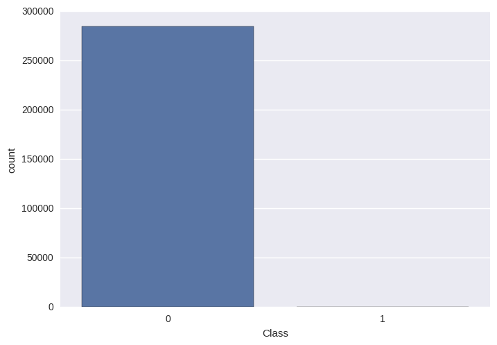
Since they are unequal, we can use upsampling
data, test_data = UpSample(x, y)
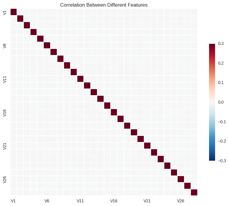
Now we can look for correlations in the data
X_data = card_data.iloc[:,1:29]

# Correlation matrix for margin features

corr = X_data.corr()

# Set up the matplotlib figure
plt.clf()
plt.subplots(figsize=(10,10))

# Draw the heat map
sns.heatmap(corr, vmax=0.3, square=True, xticklabels=5, yticklabels=5, linewidths=0.5, cbar_kws={"shrink": 0.5})

plt.title("Correlation Between Different Features")
<matplotlib.text.Text at 0x7fafbd1f6668>


<matplotlib.figure.Figure at 0x7fafc6007b00>
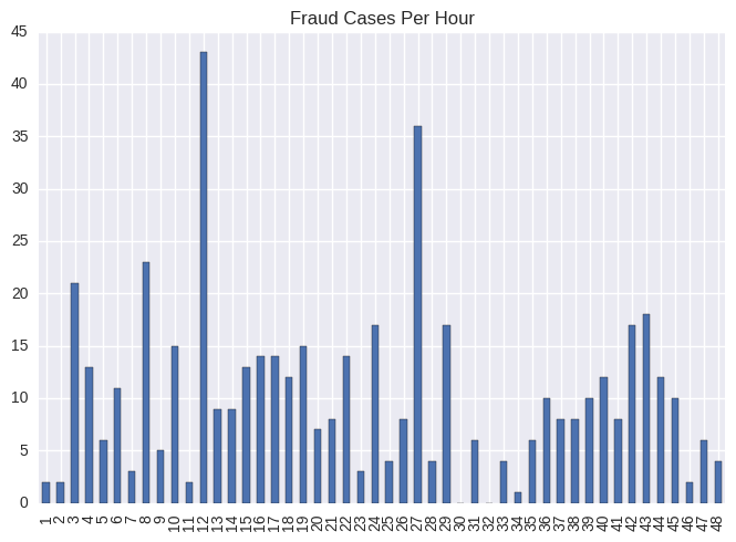
Finally, we can see the correlation of the number of fraud cases per hour
fraud = card_data.loc[card_data["Class"] == 1]
per_bins = 3600
bin_range = np.arange(0, 172801, per_bins)

out, bins = pd.cut(fraud["Time"], bins=bin_range, include_lowest=True, right=False, retbins=True)

out.cat.categories = ((bins[:-1]/3600)+1).astype(int)
out.value_counts(sort=False).plot(kind="bar", title="Fraud Cases Per Hour")
<matplotlib.axes._subplots.AxesSubplot at 0x7fafc5faf320>
Now we can run the classifiers to predict the classes
Support Vector Machines
svm = LinearSVC()
svm.fit(data[0], data[1])
y_pred = svm.predict(test_data[0])
print(classification_report(y_pred, test_data[1]))
             precision    recall  f1-score   support

        0.0       0.98      1.00      0.99     55690
        1.0       0.82      0.06      0.12      1274

avg / total       0.98      0.98      0.97     56964
Logistic Regression
log_reg = LogisticRegressionCV()
log_reg.fit(data[0], data[1])
y_pred = log_reg.predict(test_data[0])
print(classification_report(y_pred, test_data[1]))
             precision    recall  f1-score   support

        0.0       0.99      1.00      0.99     56315
        1.0       0.86      0.13      0.23       649

avg / total       0.99      0.99      0.99     56964
Gaussian Naive Bayes
gnb = GaussianNB()
gnb.fit(data[0], data[1])
y_pred = gnb.predict(test_data[0])
print(classification_report(y_pred, test_data[1]))
             precision    recall  f1-score   support

        0.0       0.99      1.00      1.00     56432
        1.0       0.68      0.13      0.22       532

avg / total       0.99      0.99      0.99     56964
In these tests, Logistic Regression outperformed both Linear SVM and Naive Bayes. This is most likely due to the fact that Logistic Regression performs well with uneven data sets, and also that there is probably some correlation between the features, reducing the effectiveness of Gaussian Naive Bayes.
Also, in looking at the results for each of these, the low values for recall and f1-score are not really relevant for the fraud causes. The reason is as follows:
Recall is defined by the following function
where stands for “true positive” and stands for “false negative.” While the accuracy for the cases that wasn’t fraud detection was on the order of 99% accurate, this leaves approximately 1% being mislabeled. Due to the above definition of recall, this will greatly inflate the denominator since the number of mislabelled non-fraud transactions would be quite large compared to the total number of actual fradulent transactions.
The same goes for the f1-score for the fraud transacations since the F1 score is defined as
Since recall is a multiplied factor in the numerator, it skews the results here as well.