Predicting Air Quality

For this project, I will be using two regression techniques, KNN Regression and Multivariate Linear Regression. The difference is that I’m going to be using Multivariate Linear Regression, instead of Univariate Linear Regression like I discussed in my previous post.

Multivariate Linear Regression

Multivariate linear regression is very similar to Univariate, the only difference is that we have more variables/features and more derivatives to take. Our hypothesis function can be represented as

$$h_{\theta}(x) = \theta_{0} + \sum_{i=1}^{M}\theta_{i}x_{i}$$

where $x_{0} = 1$, $\vec{\theta} \in \mathbb{R}^{M+1}$, and $\vec{x} \in \mathbb{R}^{M+1}$. This means that we can rewrite our function as

$$h_{\theta}(\vec{x}) = \vec{\theta}^{T}\cdot \vec{x}$$

where it is just a resulting vector inner-product. From here, there are two ways we can solve this. One is by Gradient Descent but also by the Normal Equation.

Multivariate Gradient Descent

Our cost function is similar to that in univariate gradient descent, and is

$$J(\vec{\theta}) = \frac{1}{2N}\sum_{i=1}^{N}\left[ h_{\theta}\left(x^{(i)}\right) - y^{(i)} \right]^{2}$$

where $J$ is a function of the parameter vector, $\vec{\theta}$ rather than only two $\theta$ parameters as the last time.

How we’re going to implement Gradient Descent is

$$\theta_{j} = \theta_{j} - \alpha \frac{\partial}{\partial \theta_{j}}J(\vec{\theta})$$

where $j \in \{ 0, 1, \ldots, m\}$ since there is one for each feature. We also want to update each $\theta$ simultaneously, just like before since we don’t want to update $\theta_{j}$ until the next iteration. The partial derivative terms follow the form

$$\frac{\partial}{\partial \theta_{j}} = \frac{1}{N} \sum_{i=1}^{N}\left[h_{\theta}\left( x^{(i)}\right) - y^{(i)} \right]x_{j}^{(i)}$$

which we can plug back into our equation above, giving

$$\theta_{j} = \theta_{j} - \alpha \frac{1}{N}\sum_{i=1}^{N}\left[h_{\theta}\left( x^{(i)}\right) - y^{(i)} \right]x_{j}^{(i)}$$

Feature Scaling

For a problem with multiple features, we need to make sure that the features are on a similar scale (i.e. ranges of values). This will allow Gradient Descent to converge quicker.

Example:

Let’s say you have a feature vector for a house. And your two features are $x_{1} = \text{size } (0 - 2000 ft^{2})$ and $x_{2} = \text{bedrooms } (1-5)$.

If you plot the contours of $J(\vec{\theta})$, they will be skewed and more elliptically shaped, and it can oscillate back and forth until it locates the global minimum.

Therefore, the way to fix this is to scale all the features to the same ranges. We can simply go through the data and manipulate it by

$$x_{1} = \frac{\text{size }ft^{2}}{2000}$$ $$x_{2} = \frac{\text{bedrooms}}{5}$$

This will allow Gradient Descent to take a much more direct path to the minimum, and it will converge much quicker.

We can also use a “mean normalization approach” for feature scaling, where we make the mean be at 0, thus giving a feature range of $-1 \leq x_{i} \leq 1$. From our above example, this would translate to

$$x_{1} = \frac{\text{size} - 1000}{2000}$$ $$x_{2} = \frac{\text{bedrooms} - 2}{5}$$

Note: It does not have to be exactly in the same ranges, as long as the ranges are in the same magnitude.

This can be generalized to be

$$x_{i} = \frac{x_{i} - \mu_{i}}{\sigma_{i}}$$

where $\mu_{i}$ is the average and $\sigma_{i}$ is either the standard deviation of the range of values, or it can simply be set to $max - min$.

Polynomial Regression

Polynomial regression will allow you to fit much more complicated functions with following a similar format to linear regression.

This will allow you to create your own feature, rather than just using what was given. This is useful if you have some insight about the problem and the features you think would be better suited for your problem. For example, consider the figure below

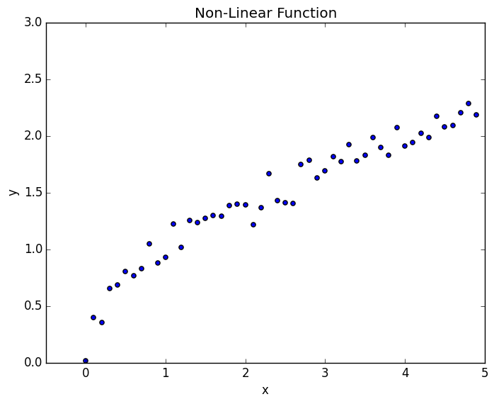
It is obviously a non-linear function. However, we can tell that it at least looks somewhat like $\sqrt{x}$ from the data. We can make our hypothesis function

$$h_{\theta}(x) = \theta_{0} + \theta_{1}\sqrt{x_{1}}$$

and we can use the normal routine that we use for linear regression. In doing so, the results are

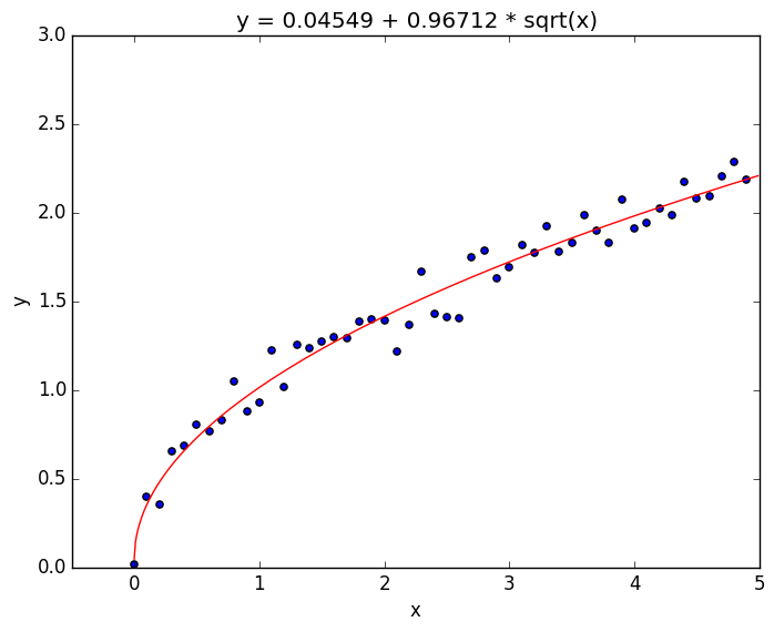
This can easily be extended to different powers of $x$ by simply changing $h_{\theta}(x)$.

The python script used to generate these plots can be found here.

Normal Equation

The normal equation is good for various problems in giving the minimum of the function. The normal equation gives us a way to solve for $\vec{\theta}$ analytically, and not have to worry about iterations to get to the solution. Because it gives the exact solution, you don’t need to worry about feature scaling as you do with Gradient Descent.

The idea for this equation is that we take the derivative of $J(\vec{\theta})\ \forall \ j$ and set all the equations equal to zero and solve. As from Calculus, this would give the minimum of the function. The results from doing this is

$$\vec{\theta} = \left( X^{T}X \right)^{-1}X^{T} \vec{y}$$

where $X$ is a matrix with each row representing a feature vector, and $\vec{y}$ is a vector where each row represents the corresponding “true value.”

There are a few potential problems with this technique. It is usually fast, though becomes slow and memory intensive for large feature vectors. Therefore, for larger problems, Gradient Descent is better to be used, while the Normal Equation excels in smaller types of problems. The order of magnitude where you should be considering switching to Gradient Descent is for problems where your $X$ is somewhere on the order of $10000 \times 10000$. Most modern day computers can do larger linear algebra routines below this quick enough to where it won’t be too memory intensive or take too long.

The other problem is with linearity of the matrix. There is no guarentee that $X$ is singular (invertible). This has the potential to cause problems when calculating $(X^{T}X)^{-1}$. Instead of calculating the inverse directly, what you can do is use the “Pseudoinverse” which will give you a good enough representation of the inverse every time and it will be close enough for the problem. The pseudoinverse can be implemented in numpy with the use of numpy.linalg.pinv(). This is also fixed with the use of regularization which is discussed in a later post.

Air Quality Prediction

The code for this project can be found here.

Cleaning the Data

The data had to be “cleaned” since it had some features which were missing in the original data set. To do so, there were two different parameters that were used. First, if a data point had more than 2 features missing, that data was thrown out. Second, to make up for the missing features, KNN Regression with k = 3 was used to get the 3 closest neighbors. From here, the missing feature was filled in with the average of the three closest neighbors.

In calculating the nearest neighbors, only those datasets with all features were used. This may not have been the best thing to do since there were only approximately 900 data points that had all the features, while there were around 7,000 data points with only 1 or two missing features.

Modeling the data

The method used was the Normal Equation which is stated above. This was so that things such as “feature scaling” wouldn’t have to be dealt with, and also the matrix was small enough $(7,300 \times 14)$ which would not be too computationally intensive for the linear algebraic operations. The normal equation was used a total of 10 times, once for each of the features that were being modeled.

In looking at the data, it seemed mostly linear throughout the course of the day, therefore a linear function was used, one value of $\theta$ for each feature. The features that were used had the values:

1. 1 (Offset)
2. Month
3. Day
4. Year
5. Time (Hour)
6. Temperature in °C
7. Relative Humidity (%)
8. AH Absolute Humidity
9. Monday (boolean)
10. Tuesday (boolean)
11. Wednesday (boolean)
12. Thursday (boolean)
13. Friday (boolean)
14. Saturday (boolean)
15. Sunday (boolean)

Where the last 7 features were created from the date. The logic behind using these was that during the week there should be more pollution in the air and this should hopefully be able to act as a relative attribute without having direct features for number of people driving, factories, etc.

After training the model, it was tested on predicting the values of the last 24 hours in the data set. The “true values” of the concentrations can be seen below

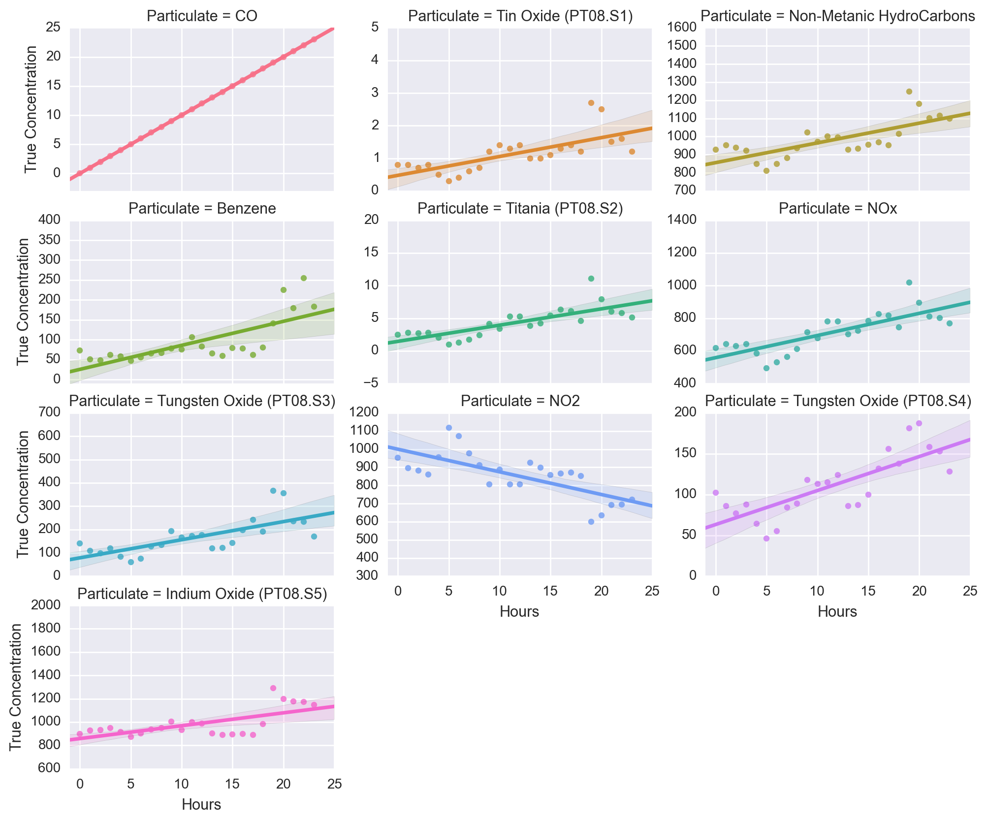
As can be seen, the data seems to be mostly linear relative to the hours. In using the model to predict the final 24 hours, we get concentration values such as

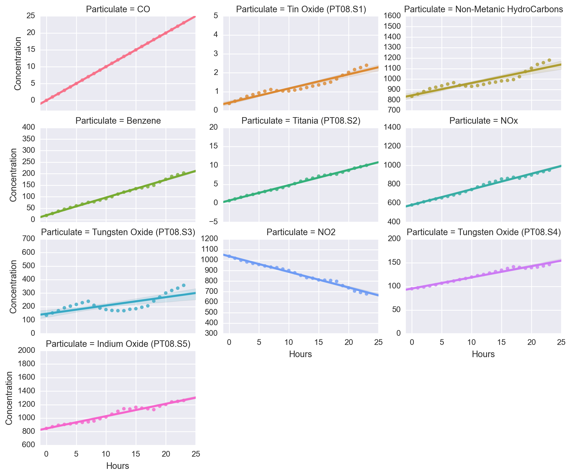
Which, at least in two dimensions seems to be mostly linear in time. It also seems to agree quite well with the trends in the actual results above.

Following this, we can look at the relative error of the data. Over the last 24 hours, the relative error for each of the particulates can be seen below.

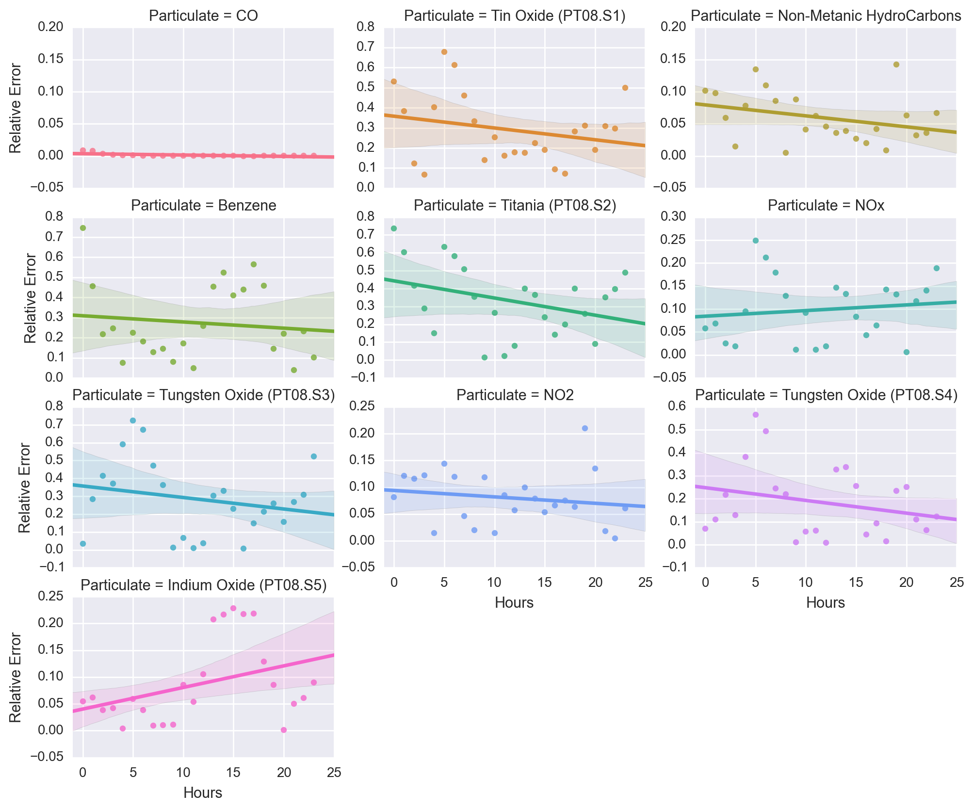
As this figure shows, the relative error did quite well for CO, and even for Non-Metanic HydroCarbons, NO2, NOx, and Indium Oxide (PT08.S5), as all of these had a maximum trendline in their relative error at 10% or less.

However, the other particulates have a much more varied response in their relative errors. This is possibly due to not having enough features to account for these. For example, a feature of wind speed and direction could be useful as that is an important factor when it comes to pollution. As well as if it rained or not (and how much) as that helps with mitigating pollution as well.

To get a better picture of the pollution, we can look at the distribution of the relative errors, which can be seen below.

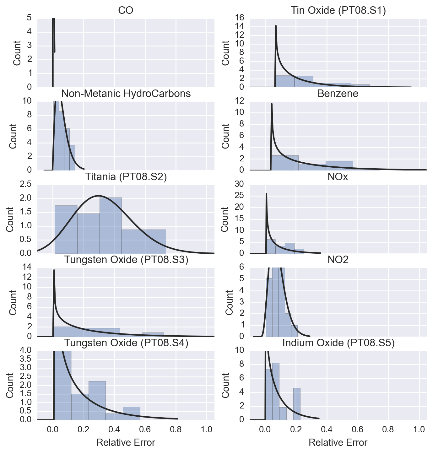
This plot shows that the most common average relative error is around 20% or less, which is a decent model for predicting the data considering that there are other features that could have helped improve this model.