Linear Regression

Linear Regression is one of the most used algorithms when it comes to regression in machine learning practices. Linear Regression treats each feature of the input feature vector as having a linear dependence on the regression model.

For example, imagine that you have some data such as height and age of various people. Something that looks like

x: Age (years)	y: Height (meters)
2.0659	0.7919
2.3684	0.9160
2.5400	0.9054
…	…

And so on, producing a plot of

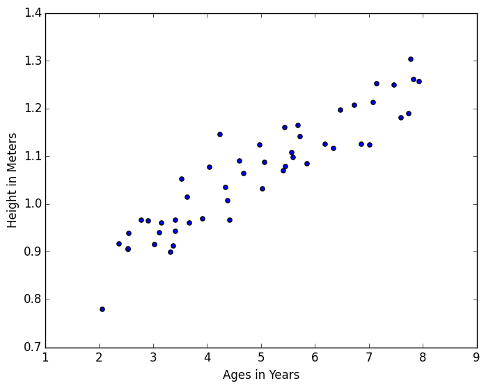
Now let’s say that given a certain age, you want to predict the height in meters from this data. This data would be considered your “training set,” and would be used to train your linear regression classifier so that you can predict results.

What it would essentially do is give you a linear fit based on some given parameter, which in this instance would be the age. In other words, it maps values from $x$ to $y$.

Univariate Linear Regression

For everything in the 1-Dimensional case, the data and corresponding code that I write can be found here, which contains the entire dataset from the plot above which will be used in this exploration of linear regression.

As stated before, we want our linear regression model to essentially be able to predict a value based on a given input parameter $x$. In other words, since it is a linear model, we want some hypothesis function

$$h_{\theta}(x) = \theta_{0} + \theta_{1}x$$

where $\theta_{0}$ is the “offset” of our function. As you can see, the above equation is linear in $x$. Essentially what we’re going to get is a straight line that fits the data above. We can do this with a cost function.

Cost function

We want to choose $\theta_{0}$ and $\theta_{1}$ such that $h_{\theta}(x)$ is close to $y$ for our training examples $(x,y)$. More formally, we want to solve

$$\min_{\theta_{0},\theta_{1}} \frac{1}{2N}\sum_{i=1}^{N}\left[ h_{\theta}\left(x^{(i)}\right) - y^{(i)} \right]^{2}$$

Where we’re going to be minimizing the average difference, hence the fractional value out front.

Using this above equation, we can define it as a function to determine the best values, namely

$$J(\theta_{0}, \theta_{1}) = \frac{1}{2N}\sum_{i=1}^{N}\left[ h_{\theta}\left(x^{(i)}\right) - y^{(i)} \right]^{2}$$

where $J(\theta_{0}, \theta_{1})$ is our cost function. We want to use our cost function to solve

$$\min_{\theta_{0},\theta_{1}} J(\theta_{0}, \theta_{1})$$

which is a minimization problem. This can be done with the Method of Gradient Descent.

Batch Gradient Descent

The generalized steps of Gradient Descent is we have some function $J(\vec{\theta})$ (note, it can be multivariate) and we want to minimize it over all values of $\theta_{i}$.

In our example, we will only be using it for the 1-diemsional case, i.e. $\theta_{0},\ \theta_{1}$. The outline of the algorithm is:

1. Start with some values of $\theta_{0}$ and $\theta_{1}$
2. Keep changing $\theta_{0}$ and $\theta_{1}$ to reduce $J(\theta_{0}, \theta_{1})$ until we hopefully end at the minimum

How gradient descent works, is it traverses towards the path of greatest descent to try and minimize the function. It attempts to find the path of quickest descent to the minima or at the very least the local minima. At which point, it has “converged.”

Mathematically, this can be written as

$$\theta_{j} = \theta_{j} - \alpha\frac{\partial}{\partial \theta_{j}}J(\vec{\theta})$$

for all $j \in \{0, 1, \ldots, M\}$, where $M$ is the size of your feature vector, which for this 1D case would be $\{ 0, 1\}$. You would repeat the above equation until convergence is reached. You should be updating $\theta_{i}$ simultaneously, meaning you calculate for all values of $\theta_{i}$, and only after are the updates performed.

In the above equation, $\alpha$ is known as your learning rate which denotes how fast the function will converge. However, if this learning rate is too high, it’s possible that the function will never reach a minimum anywhere and will never converge. However, if it is too small, it can take a while to converge.

We can apply this to our cost function, but we need to determine what the partial derivative is. For $\frac{\partial}{\partial \theta_{0}}$ we get

$$\frac{\partial}{\partial \theta_{0}}J(\theta_{0}, \theta_{1}) = \frac{1}{N}\sum_{i=1}^{N}\left[ h_{\theta}\left( x^{(i)}\right) - y^{(i)}\right]$$

and for $\frac{\partial}{\partial \theta_{1}}$

$$\frac{\partial}{\partial \theta_{1}}J(\theta_{0}, \theta_{1}) = \frac{1}{N}\sum_{i=1}^{N}\left[ h_{\theta}\left( x^{(i)}\right) - y^{(i)}\right]x^{(i)}$$

where $N$ is your training set. Our Gradient Descent algorithm becomes

$$\theta_{0} = \theta_{0} - \alpha\frac{1}{m}\sum_{i=1}^{N}\left[ h_{\theta}\left( x^{(i)}\right) - y^{(i)}\right]$$ $$\theta_{1} = \theta_{1} - \alpha\frac{1}{N}\sum_{i=1}^{N}\left[ h_{\theta}\left( x^{(i)}\right) - y^{(i)}\right]$$

Where we perform a “simultaneous update” over the values of the feature vector.

Applying to Age and Height Data

We can use this above technique to find a linear regression line over this data to find out the best fit for the data so we can approximate a height given an age.

Again, the code can be found here, which reads in the data and performs the linear regression using gradient descent.

The above defined algorithms were used and implemented, where it would simultaneously update the values of $\theta_{0}$ and $\theta_{1}$. It would continually do this until the condition $\left\| \vec{\theta} - \vec{\theta}_{old} \right\| _{2} < 10^{-6}$ was met.

I chose a value of $\alpha = 0.25$ for this problem, and also stored all the values of $\vec{\theta}$ so you can see how $\vec{\theta}$ evolves over time.

The final result of this was

$$\vec{\theta} = \begin{pmatrix}0.75101\\ 0.06370 \end{pmatrix}$$

where you can see the evolution of $\vec{\theta}$ as it evolves below.